Probability and Distribution
大约 13 分钟
Probability and Distribution
Probability

Random
# 设置随机数种子
np.random.seed(10)
# replace = True 表示允许重复取值, 即取出后放回
sales_counts.sample(5, replace = True)
name 	n_sales
1 		Brian 128
2 		Claire 75
1 		Brian 128
3 		Damian 69
0 		Amir 178
- Independent events: 如果第二个事件的概率不受第一个事件的结果影响,那么两个事件就是独立的。
- Sampling with replacement = each pick isindependent
- Dependent events: 如果第二事件的概率受第一个事件的结果影响,则两个事件取决于两个事件。
- Sampling with replacement = each pick isindependent
Law of large numbers
随着你的样本量的增加,样本的平均值将接近预期值。
Central Limit Theorem
样本的平均值、方差和中位数等描述性数据可用于描述总体数据。
中心极限定理适用于各种分布(without replacement)。 无论您从中采取样品平均值的分布形状如何,如果采样分布包含足够的样品均值,则中央限制定理将适用。
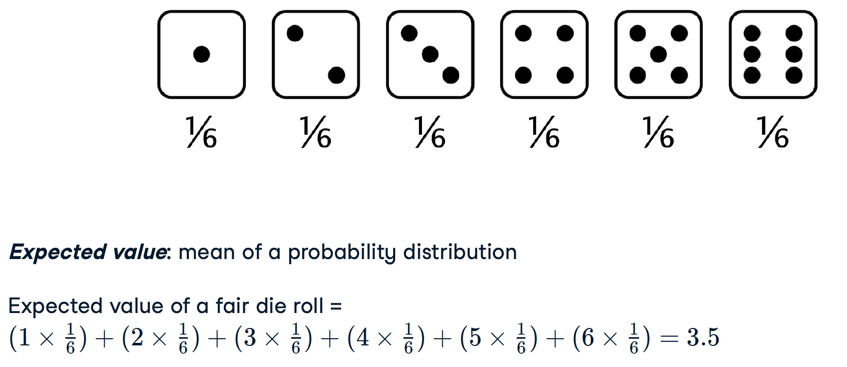
Discrete distributions
Uniform distribution
描述了一个场景中每种可能结果的概率
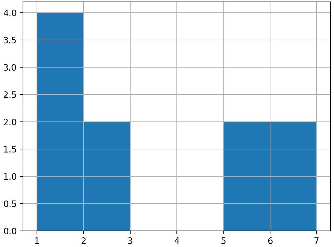
rolls_10 = die.sample(10, replace = True)
rolls_10
		number
0 	1
0 	1
4 	5
1 	2
0 	1
0 	1
5 	6
5 	6
...
rolls_10['number'].hist(bins=np.linspace(1,7,7))
plt.show()
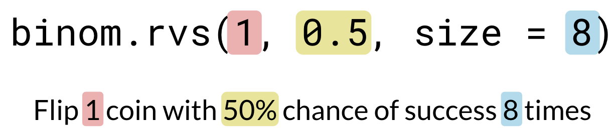
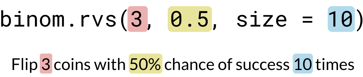
Binomial distribution
如果试验不是独立的,那么二项分布就不适用。当样本足够多时,也可以把非独立实验当做二项分布。
随机取样

1 = head, 0 = tails
from scipy.stats import binom
binom.rvs(1, 0.5, size=1)
binom.rvs(1, 0.5, size=8)
binom.rvs(8, 0.5, size=1)
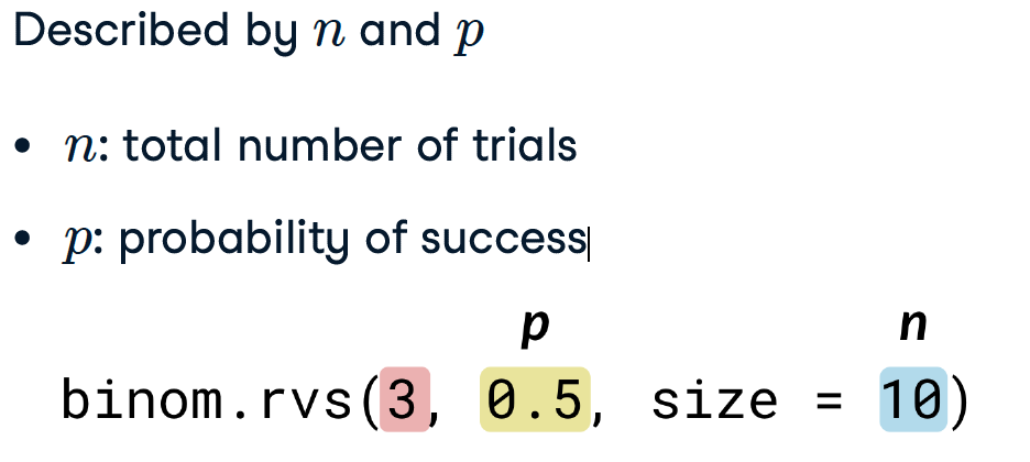
binom.rvs(3, 0.5, size=10)
array([1])
array([0, 1, 1, 0, 1, 0, 1, 1])
array([5])
array([0, 3, 2, 1, 3, 0, 2, 2, 0, 0])

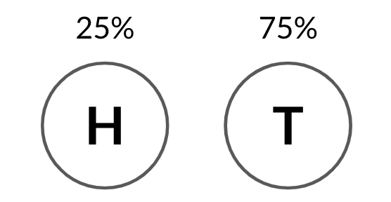
binom.rvs(3, 0.25, size=10)
array([1, 1, 1, 1, 0, 0, 2, 0, 1, 0])
计算概率
Binomial distribution「二项分布」 是 一系列独立试验中成功次数的概率分布
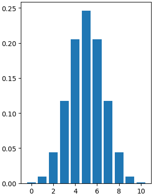
# binom.pmf(num heads, num trials, prob of heads) -> 10C7
# P (heads = 7)
binom.pmf(7, 10, 0.5)

# P (heads ≤ 7)
binom.cdf(7, 10, 0.5)
0.1171875
0.9453125
Expected value
- Expected value = n × p
- Expected number of heads out of 10 fips = 10 × 0.5 = 5
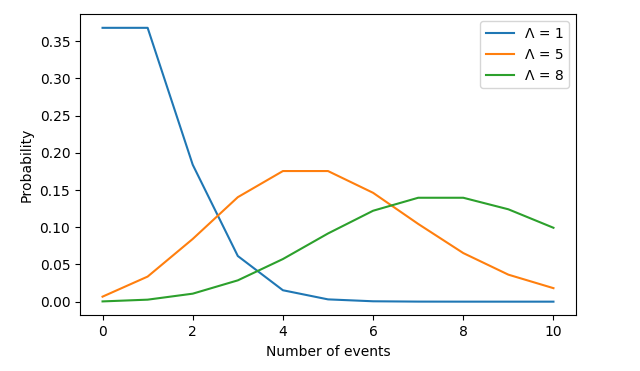
Poisson distribution
事件似乎以一定的速度发生,但完全是随机的
例子
- 每周从动物收容所收养的动物数量
- 每小时到达一家餐馆的人数
- 加州每年发生的地震数量
时间单位无关紧要,只要你在谈论同样的情况时使用相同的单位即可。
泊松分布适用于在一个固定的时间段内,一些事件发生的概率。
例子
- 每周从动物收容所收养≥5只动物的概率
- 一家餐馆每小时有12人到达的概率
- 加州每年发生<20次地震的概率
Lambda is the distribution's peak
# 如果每周平均收养人数为8,那么P是多少(#一周内收养人数=5)?
from scipy.stats import poisson
poisson.pmf(5, 8)

# 如果每周平均收养人数为8,那么P(#一周内收养人数≤5)是多少?
poisson.cdf(5, 8)
0.09160366
0.1912361
Continuous distributions

Uniform distribution
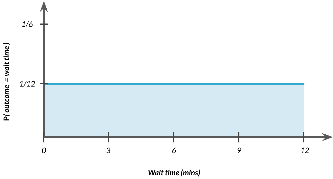
# P (wait time ≤ 7)
from scipy.stats import uniform
uniform.cdf(7, 0, 12)

# P (wait time ≥ 7) = 1 − P (wait time ≤ 7)
from scipy.stats import uniform
1 - uniform.cdf(7, 0, 12)
0.5833333
0.4166667
# Generating random numbers according to uniform distribution
from scipy.stats import uniform
uniform.rvs(0, 5, size=10)
array([1.89740094, 4.70673196, 0.33224683, 1.0137103 , 2.31641255, 3.49969897, 0.29688598, 0.92057234, 4.71086658, 1.56815855])
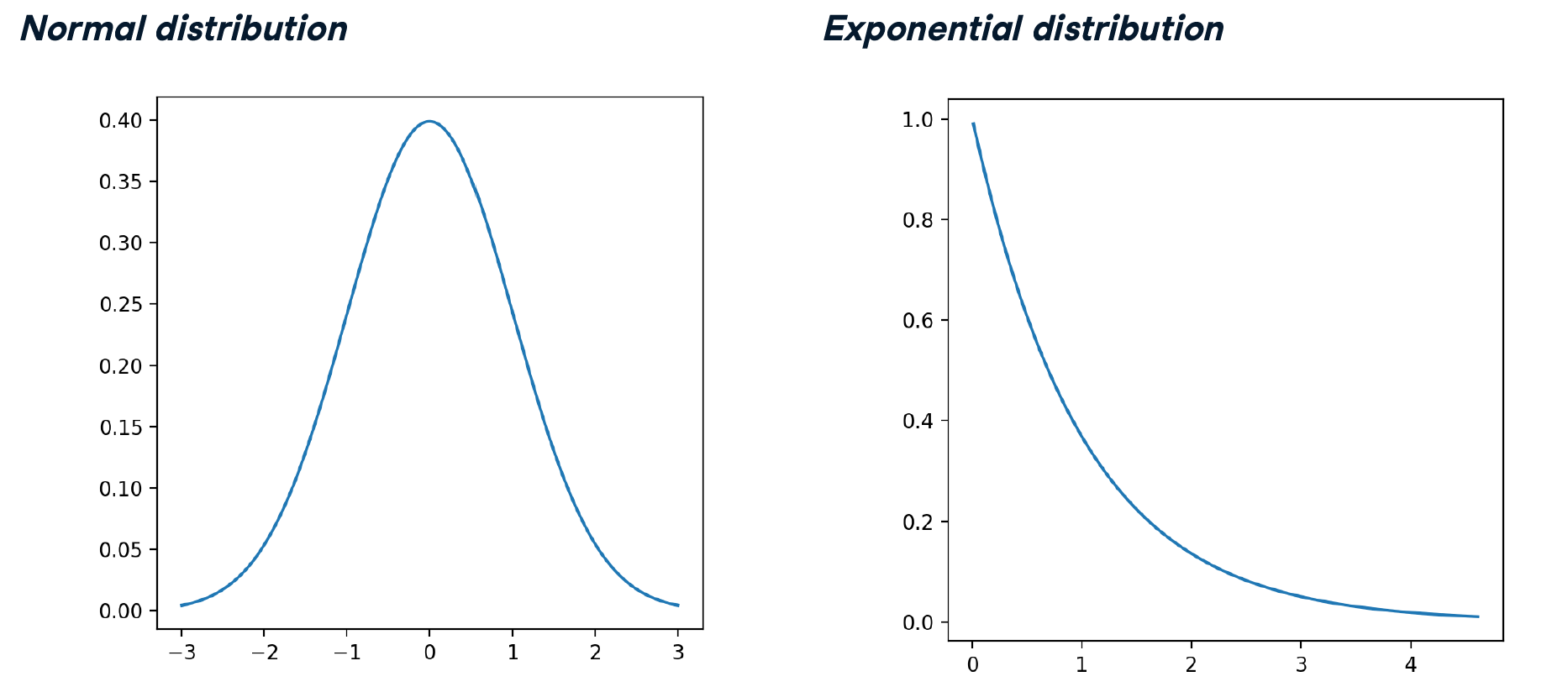
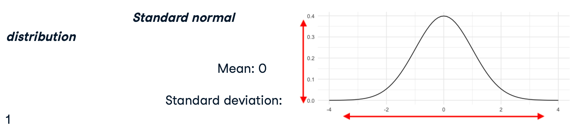
Normal distribution
- means = μ
- std = σ
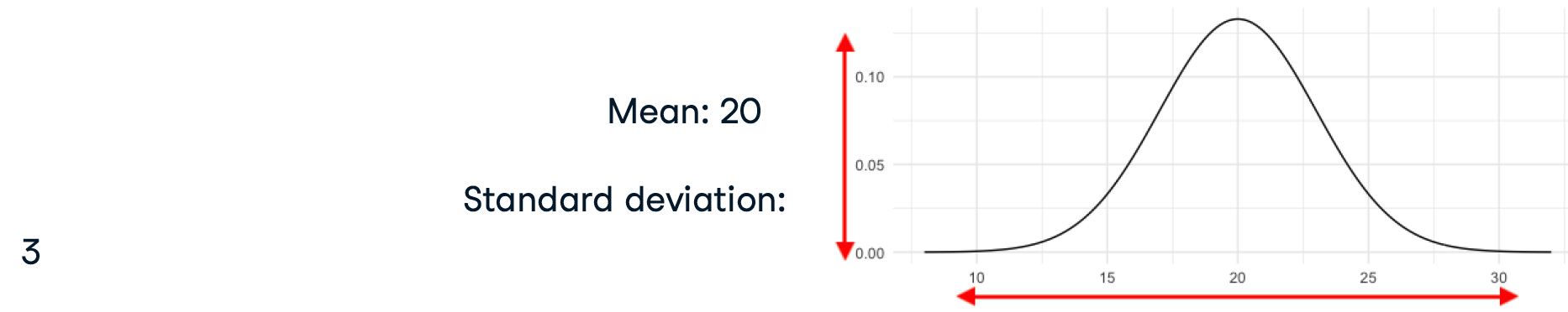
标准正态分布
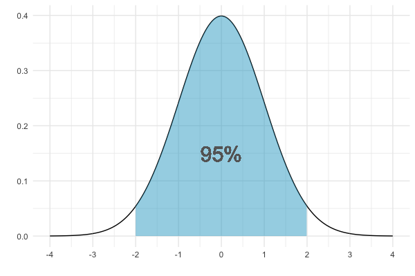
99-95-86定则
- 68% falls within 1 standard deviation
- 95% falls within 2 standard deviations
- 99.7% falls within 3 standard deviations
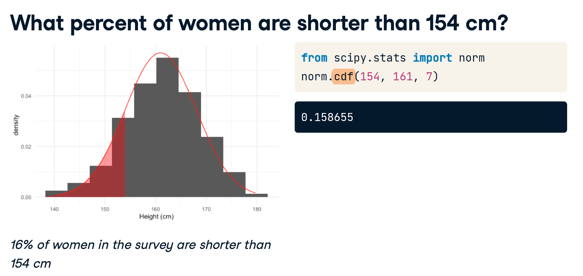
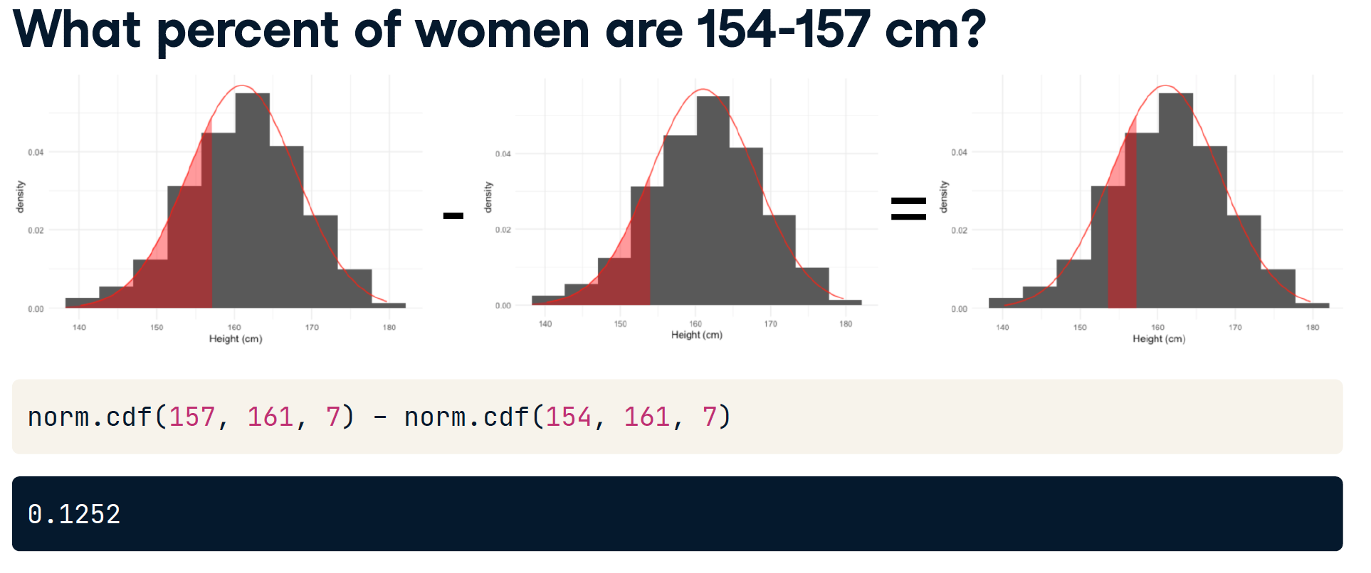
计算概率
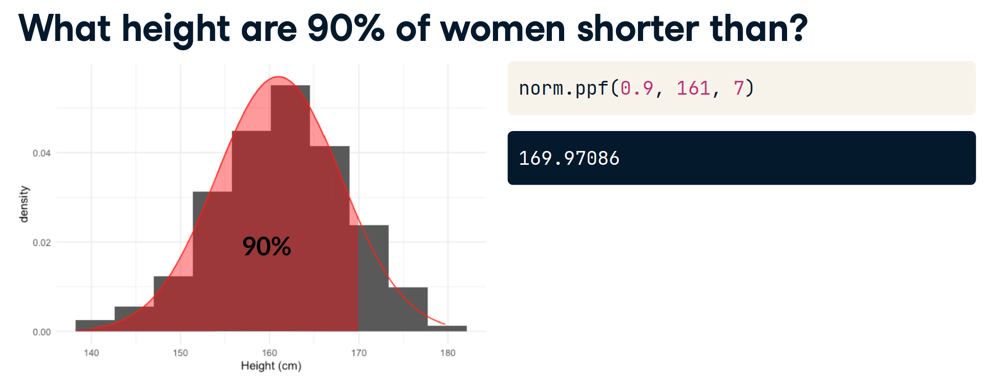
Generating random numbers
# Generate 10 random heights
norm.rvs(161, 7, size=10)
array([155.5758223 , 155.13133235, 160.06377097, 168.33345778, 165.92273375, 163.32677057, 165.13280753, 146.36133538, 149.07845021, 160.5790856 ])

Exponential distribution
泊松事件之间的时间概率
例子
- 两次收养之间的概率>1天
- 餐馆到达之间的概率<10分钟
- 地震间隔6-8个月的概率
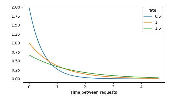
Also uses rate = 1/lambda
- lambda: 单位时间多少个
- rate:产生一平均需要多长时间
举例: λ = 0.5, 每分钟创建 0.5 张客户服务单 - > rate = 2, 平均每 2 分钟就有一张客户服务单产生
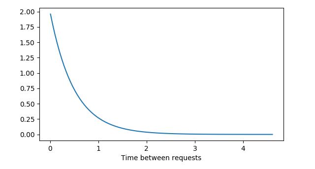
Lambda in exponential distribution
计算概率
from scipy.stats import expon
# 假设 rate = 0.5
# P (wait < 1 min) =
expon.cdf(1, scale=0.5)
0.8646647167633873
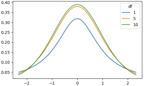
(Student's) t-distribution
与正态分布的形状相似
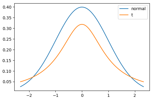
自由度
- 有自由度参数(df),它决定了尾巴的厚度。
- 较低的df = 较厚的尾部,较高的标准差
- 较高的df = 更接近正态分布
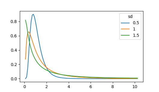
Log-normal distribution
Variable whose logarithm is normally distributed
Examples:
- Length of chess games
- Adult blood pressure
- Number of hospitalizations in the 2003 SARS outbreak